In the previous article, we delved deeply into slices, comparing arrays, lists, strings, and their relationships with slices and slice references. Today, we will continue discussing another extremely important collection container in Rust: HashMap, or hash tables.
If we talk about the most important and frequently appearing data structures in software development, hash tables definitely rank among them. Many programming languages even incorporate hash tables as a built-in data structure into the core of the language. For example, PHP’s associative array, Python’s dict, JavaScript’s object and Map.
In a CppCon 2017 talk by Google engineer Matt Kulukundis, it was mentioned that 1% of CPU time on Google’s servers worldwide is spent on hash table computations, and over 4% of memory is used to store hash tables. This sufficiently demonstrates the importance of hash tables.
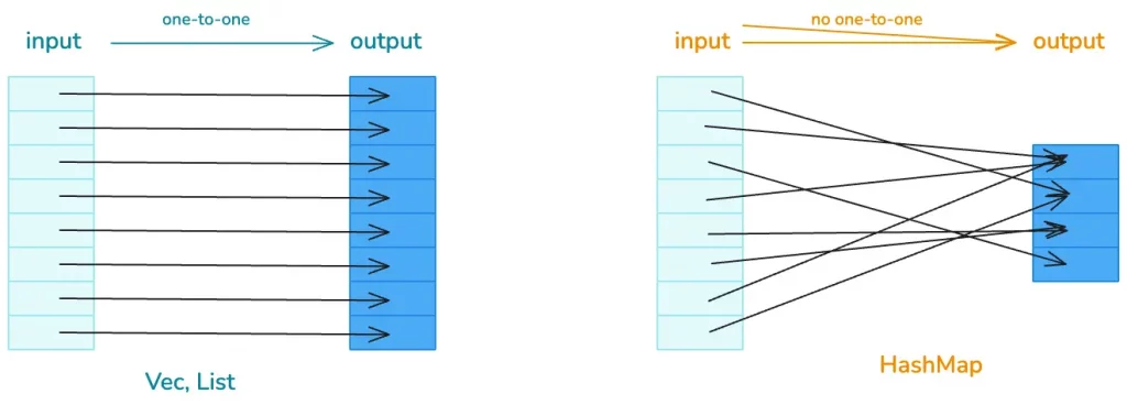
We know that hash tables are similar to lists, both used to handle data structures that require random access. If the input and output of the data structure have a one-to-one correspondence, lists can be used; if there is no one-to-one correspondence, then hash tables are needed.
Rust’s Hash Table
So, what kind of hash table does Rust provide for us? What does it look like? What is its performance? Let’s start learning from the official documentation.
If you open the HashMap documentation, you will see this sentence:
A hash map implemented with quadratic probing and SIMD lookup.
This immediately raises some adrenaline, as two high-end terms appear: quadratic probing and SIMD lookup. What do they mean? They are the core design of Rust’s hash table algorithm, and our study today will revolve around these two terms. So don’t worry, after learning, I believe you will understand this sentence.
Let’s first go through the basic theory. The most core characteristic of a hash table is: a huge number of possible inputs and a limited hash table capacity. This leads to hash collisions, meaning two or more inputs are hashed to the same location, so we need to be able to handle hash collisions.
To resolve collisions, we can first use better, more evenly distributed hash functions and larger hash tables to mitigate conflicts, but this cannot completely solve the problem, so we also need to use collision resolution mechanisms.
How to resolve collisions?
Theoretically, the main collision resolution mechanisms are chaining and open addressing.
Chaining is familiar to us; it involves linking data that falls into the same hash using a singly or doubly linked list. When searching, the corresponding hash bucket is found first, and then the collision chain is compared one by one until a matching item is found:
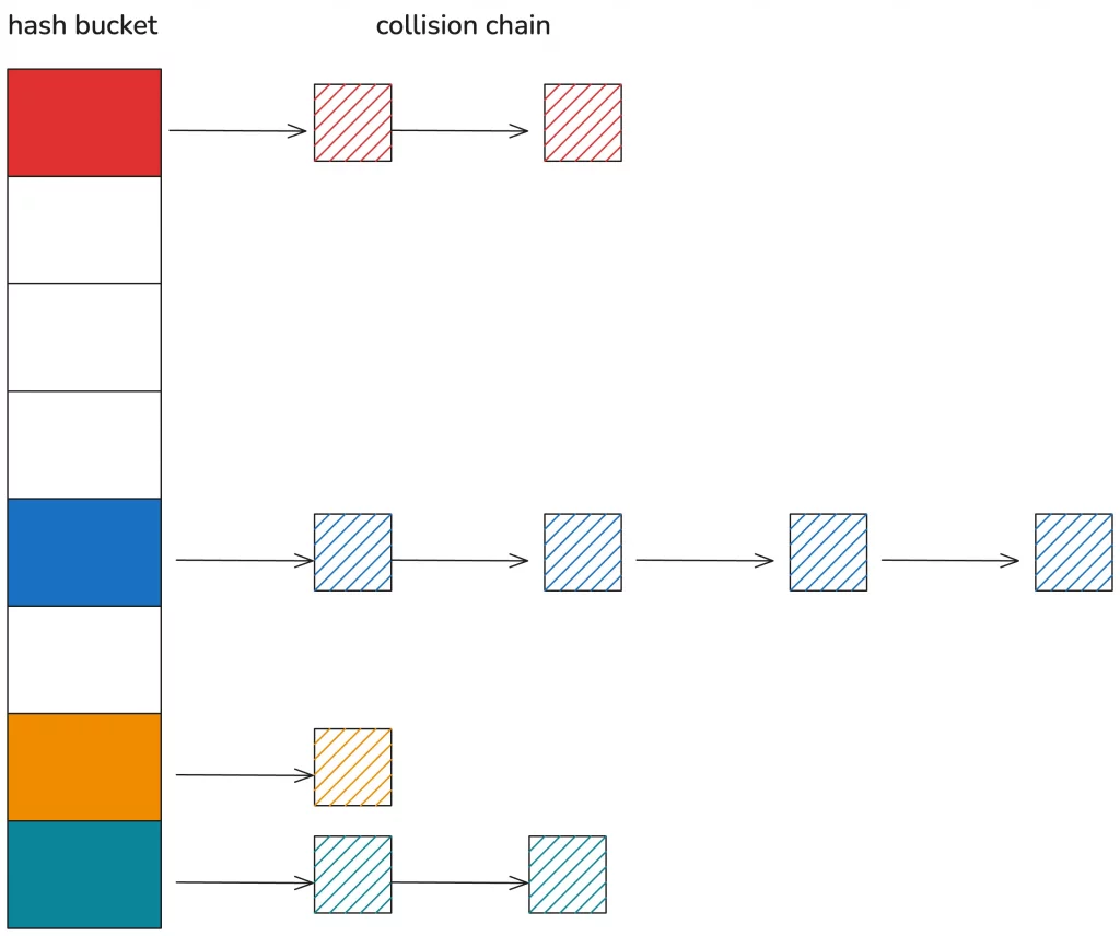
Chaining handles hash collisions very intuitively, making it easy to understand and write code, but the disadvantage is that the hash table and the collision chain use different memory, which is not cache-friendly.
Open addressing treats the entire hash table as a large array without introducing additional memory. When a collision occurs, data is inserted into other free positions according to certain rules. For example, linear probing, when a hash collision occurs, continuously probes backward until a free position is found for insertion.
Quadratic probing, theoretically, when a conflict occurs, continuously probes the hash position plus or minus n squared to find a free position for insertion. Let’s look at the diagram for easier understanding:
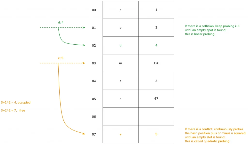
(The diagram illustrates the theoretical processing method; in practice, there are many different treatments for performance.)
Open addressing has other schemes, such as double hashing, which we won’t detail today.
Okay, understanding the theoretical knowledge of quadratic probing for hash tables, we can infer that Rust’s hash table does not use chaining to resolve hash conflicts but uses quadratic probing in open addressing. Of course, we will later see that Rust’s quadratic probing differs somewhat from the theoretical treatment.
The other keyword, using SIMD for single instruction, multiple data lookup, is also closely related to the clever memory layout of Rust’s hash table that we will discuss shortly.
HashMap Data Structure
Getting to the main point, let’s see what the data structure of Rust’s hash table looks like. Open the source code of the standard library:
use hashbrown::hash_map as base;

#[derive(Clone)]
pub struct RandomState {
    k0: u64,
    k1: u64,
}

pub struct HashMap<K, V, S = RandomState> {
    base: base::HashMap<K, V, S>,
}
It can be seen that HashMap has three generic parameters: K and V represent the types of key/value, and S is the state of the hash algorithm, which defaults to RandomState, occupying two u64s. RandomState uses SipHash as the default hash algorithm, which is a cryptographically secure hashing function.
From the definition, we can also see that Rust’s HashMap reuses hashbrown’s HashMap. Hashbrown is an improved implementation of Google’s Swiss Table in Rust. Let’s open the hashbrown code and look at its structure:
pub struct HashMap<K, V, S = DefaultHashBuilder, A: Allocator + Clone = Global> {
    pub(crate) hash_builder: S,
    pub(crate) table: RawTable<(K, V), A>,
}
It can be seen that HashMap has two fields: one is hash_builder, of type RandomState mentioned earlier from the standard library, and the other is the specific RawTable:
pub struct RawTable<T, A: Allocator + Clone = Global> {
    table: RawTableInner<A>,
    // Tell dropck that we own instances of T.
    marker: PhantomData<T>,
}

struct RawTableInner<A> {
    // Mask to get an index from a hash value. The value is one less than the
    // number of buckets in the table.
    bucket_mask: usize,

    // [Padding], T1, T2, ..., Tlast, C1, C2, ...
    //                                ^ points here
    ctrl: NonNull<u8>,

    // Number of elements that can be inserted before we need to grow the table
    growth_left: usize,

    // Number of elements in the table, only really used by len()
    items: usize,

    alloc: A,
}
In RawTable, the actually meaningful data structure is RawTableInner. The first four fields are very important, and we will mention them again when discussing HashMap’s memory layout:
- the
usizebucket_maskis the number of hash buckets in the hash table minus one; - the pointer named
ctrlpoints to the ctrl area at the end of the hash table’s heap memory; - the
usizefieldgrowth_leftindicates how much more data the hash table can store before the next automatic growth; - the
usizeitemsindicate how much data is currently in the hash table.
The final alloc field here, like the marker in RawTable, is just a placeholder type. For now, we only need to know that it is used to allocate memory on the heap.
Basic usage methods of HashMap.
Let’s clarify the data structure first, then we’ll look at the specific usage methods. Using a Rust hash map is straightforward; it provides a series of very convenient methods, making it very similar to using them in other languages. You can easily understand it by checking the documentation. Let’s write some code to try it out:
use std::collections::HashMap;

fn main() {
    let mut map = HashMap::new();
    explain("empty", &map);

    map.insert('a', 1);
    explain("added 1", &map);

    map.insert('b', 2);
    map.insert('c', 3);
    explain("added 3", &map);

    map.insert('d', 4);
    explain("added 4", &map);

    assert_eq!(map.get(&'a'), Some(&1));
    assert_eq!(map.get_key_value(&'b'), Some((&'b', &2)));

    map.remove(&'a');

    assert_eq!(map.contains_key(&'a'), false);
    assert_eq!(map.get(&'a'), None);
    explain("removed", &map);

    map.shrink_to_fit();
    explain("shrinked", &map);
}

fn explain<K, V>(name: &str, map: &HashMap<K, V>) {
    println!("{}: len: {}, cap: {}", name, map.len(), map.capacity());
}
Running this code, we can see the following output.
empty: len: 0, cap: 0
added 1: len: 1, cap: 3
added 3: len: 3, cap: 3
added 4: len: 4, cap: 7
removed: len: 3, cap: 7
shrinked: len: 3, cap: 3
We can see that when HashMap::new() is called, it does not allocate space, the capacity is zero. As key-value pairs are continuously inserted into the hash map, it grows by powers of two minus one, with a minimum of 3. When data is removed from the table, the original table size remains unchanged. Only by explicitly calling shrink_to_fit will the hash map shrink.
The memory layout of HashMap.
However, through the public interface of HashMap, we cannot see how HashMap is laid out in memory. We still need to use the std::mem::transmute method we used before to print out the data structure. Let’s modify the previous code:
use std::collections::HashMap;

fn main() {
    let map = HashMap::new();
    let mut map = explain("empty", map);

    map.insert('a', 1);
    let mut map = explain("added 1", map);
    map.insert('b', 2);
    map.insert('c', 3);

    let mut map = explain("added 3", map);

    map.insert('d', 4);

    let mut map = explain("added 4", map);

    map.remove(&'a');

    explain("final", map);
}


fn explain<K, V>(name: &str, map: HashMap<K, V>) -> HashMap<K, V> {
    let arr: [usize; 6] = unsafe { std::mem::transmute(map) };
    println!(
        "{}: bucket_mask 0x{:x}, ctrl 0x{:x}, growth_left: {}, items: {}",
        name, arr[2], arr[3], arr[4], arr[5]
    );
    unsafe { std::mem::transmute(arr) }
}
After running it, we can see:
empty: bucket_mask 0x0, ctrl 0x1056df820, growth_left: 0, items: 0
added 1: bucket_mask 0x3, ctrl 0x7fa0d1405e30, growth_left: 2, items: 1
added 3: bucket_mask 0x3, ctrl 0x7fa0d1405e30, growth_left: 0, items: 3
added 4: bucket_mask 0x7, ctrl 0x7fa0d1405e90, growth_left: 3, items: 4
final: bucket_mask 0x7, ctrl 0x7fa0d1405e90, growth_left: 4, items: 3
Interestingly, we find that the heap address corresponding to ctrl changes during execution.
On my OS X, initially, when the hash map is empty, the ctrl address appears to be an address in the TEXT/RODATA segment, probably pointing to a default empty table address. After inserting the first data pair, the hash map allocates 4 buckets, and the ctrl address changes. After inserting three data pairs, growth_left becomes zero. Upon further insertion, the hash map reallocates, and the ctrl address changes again.
Earlier, while exploring the HashMap data structure, it was mentioned that ctrl is an address pointing to the ctrl area at the end of the hash map’s heap address. Therefore, we can calculate the starting address of the hash map’s heap memory from this address.
Because the hash map has 8 buckets (0x7 + 1), and the size of each bucket is the size of key (char) + value (i32), which is 8 bytes, the total is 64 bytes. For this example, subtracting 64 from the ctrl address gives the starting address of the hash map’s heap memory. Then, we can use rust-gdb / rust-lldb to print this memory.
Here, I use Linux’s rust-gdb to set breakpoints and check the state of the hash map with one, three, four values, and after deleting one value.
❯ rust-gdb ~/.target/debug/hashmap2
GNU gdb (Ubuntu 9.2-0ubuntu2) 9.2
...
(gdb) b hashmap2.rs:32
Breakpoint 1 at 0xa43e: file src/hashmap2.rs, line 32.
(gdb) r
Starting program: /home/tchen/.target/debug/hashmap2
...
# The initial state, the hash table is empty
empty: bucket_mask 0x0, ctrl 0x555555597be0, growth_left: 0, items: 0

Breakpoint 1, hashmap2::explain (name=..., map=...) at src/hashmap2.rs:32
32      unsafe { std::mem::transmute(arr) }
(gdb) c
Continuing.
# After inserting one element, the bucket has 4 (0x3+1), heap address start position 0x5555555a7af0 - 4*8(0x20)
added 1: bucket_mask 0x3, ctrl 0x5555555a7af0, growth_left: 2, items: 1

Breakpoint 1, hashmap2::explain (name=..., map=...) at src/hashmap2.rs:32
32      unsafe { std::mem::transmute(arr) }
(gdb) x /12x 0x5555555a7ad0
0x5555555a7ad0:  0x00000061  0x00000001  0x00000000  0x00000000
0x5555555a7ae0:  0x00000000  0x00000000  0x00000000  0x00000000
0x5555555a7af0:  0x0affffff  0xffffffff  0xffffffff  0xffffffff
(gdb) c
Continuing.
# After inserting three elements, the hash table has no remaining space, and the heap address start position remains unchanged 0x5555555a7af0 - 4*8(0x20)
added 3: bucket_mask 0x3, ctrl 0x5555555a7af0, growth_left: 0, items: 3

Breakpoint 1, hashmap2::explain (name=..., map=...) at src/hashmap2.rs:32
32      unsafe { std::mem::transmute(arr) }
(gdb) x /12x 0x5555555a7ad0
0x5555555a7ad0:  0x00000061  0x00000001  0x00000062  0x00000002
0x5555555a7ae0:  0x00000000  0x00000000  0x00000063  0x00000003
0x5555555a7af0:  0x0a72ff02  0xffffffff  0xffffffff  0xffffffff
(gdb) c
Continuing.
# After inserting the fourth element, the hash table expands, and the heap address start position changes to 0x5555555a7b50 - 8*8(0x40)
added 4: bucket_mask 0x7, ctrl 0x5555555a7b50, growth_left: 3, items: 4

Breakpoint 1, hashmap2::explain (name=..., map=...) at src/hashmap2.rs:32
32      unsafe { std::mem::transmute(arr) }
(gdb) x /20x 0x5555555a7b10
0x5555555a7b10:  0x00000061  0x00000001  0x00000000  0x00000000
0x5555555a7b20:  0x00000064  0x00000004  0x00000063  0x00000003
0x5555555a7b30:  0x00000000  0x00000000  0x00000062  0x00000002
0x5555555a7b40:  0x00000000  0x00000000  0x00000000  0x00000000
0x5555555a7b50:  0xff72ffff  0x0aff6502  0xffffffff  0xffffffff
(gdb) c
Continuing.
# After deleting 'a', there are 4 remaining positions. Note the changes in the ctrl bits, and that 0x61 0x1 have not been cleared
final: bucket_mask 0x7, ctrl 0x5555555a7b50, growth_left: 4, items: 3

Breakpoint 1, hashmap2::explain (name=..., map=...) at src/hashmap2.rs:32
32      unsafe { std::mem::transmute(arr) }
(gdb) x /20x 0x5555555a7b10
0x5555555a7b10:  0x00000061  0x00000001  0x00000000  0x00000000
0x5555555a7b20:  0x00000064  0x00000004  0x00000063  0x00000003
0x5555555a7b30:  0x00000000  0x00000000  0x00000062  0x00000002
0x5555555a7b40:  0x00000000  0x00000000  0x00000000  0x00000000
0x5555555a7b50:  0xff72ffff  0xffff6502  0xffffffff  0xffffffff
This output contains a lot of information; let’s carefully analyze it with the help of a diagram.
First, after inserting the first element ‘a’: 1, the memory layout of the hash map is as follows:
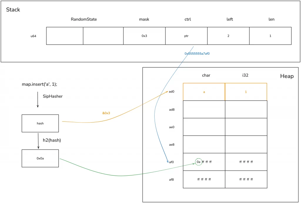
The hash of key ‘a’ is computed with the bucket_mask 0x3, resulting in position 0 for insertion. Simultaneously, the first 7 bits of this hash are taken, corresponding to position 0 in the ctrl table, and this value is written there.
The key to understanding this step is clarifying what this ctrl table is.
The ctrl table
The main purpose of the ctrl table is for fast lookups. Its design is very elegant and worth learning from.
A ctrl table contains several 128-bit or 16-byte groups, where each byte in a group is called a ctrl byte, corresponding to one bucket—so one group corresponds to 16 buckets. If the first bit of a ctrl byte corresponding to a bucket is not 1, it means that ctrl byte is in use; if all bits are 1, meaning the byte is 0xff, then it is free.
An entire set of 128 bits of control bytes can be loaded with one instruction and then masked with a certain value to find its position. This is the SIMD lookup mentioned earlier.
We know that modern CPUs support single instruction, multiple data (SIMD) operations, and Rust fully utilizes this capability of the CPU—one instruction can load multiple related data into the cache for processing, greatly speeding up table lookups. Therefore, the efficiency of Rust’s hash table lookups is very high.
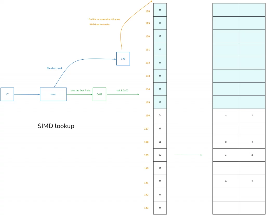
Let’s look at how HashMap uses the ctrl table for data queries. Suppose some data has already been added to this table, and we now want to find the data with the key ‘c’:
- First, hash ‘c’ to get a hash value h;
- perform a bitwise AND of h with
bucket_maskto get a value, which is 139 in the diagram; - using this 139, find the starting position of the corresponding ctrl group—since ctrl groups are in sets of 16, here we find 128;
- use a SIMD instruction to load the 16 bytes starting from the address corresponding to 128;
- take the first 7 bits of the hash and perform a bitwise AND with the 16 bytes just loaded to find the corresponding match; if found, it (they) is very likely the value being sought;
- if not, continue searching backward using quadratic probing (accumulating in multiples of 16) until found.
You can understand this algorithm with the help of the diagram below:
Therefore, when HashMap inserts and deletes data, and consequently triggers reallocation, the main work is maintaining the correspondence between this ctrl table and the data.
Because the ctrl table is the first memory touched in all operations, in the HashMap structure, the heap memory pointer directly points to the ctrl table, rather than to the start of the heap memory, to reduce one memory access.
Hash table reallocation and growth
Okay, let’s continue from where we left off regarding the memory layout. After inserting the first piece of data, our hash table only has 4 buckets, so only the first 4 bytes of the ctrl table are useful. As the hash table grows and buckets become insufficient, reallocation occurs. Since the bucket_mask is always one less than the number of buckets, reallocation happens after inserting three elements.
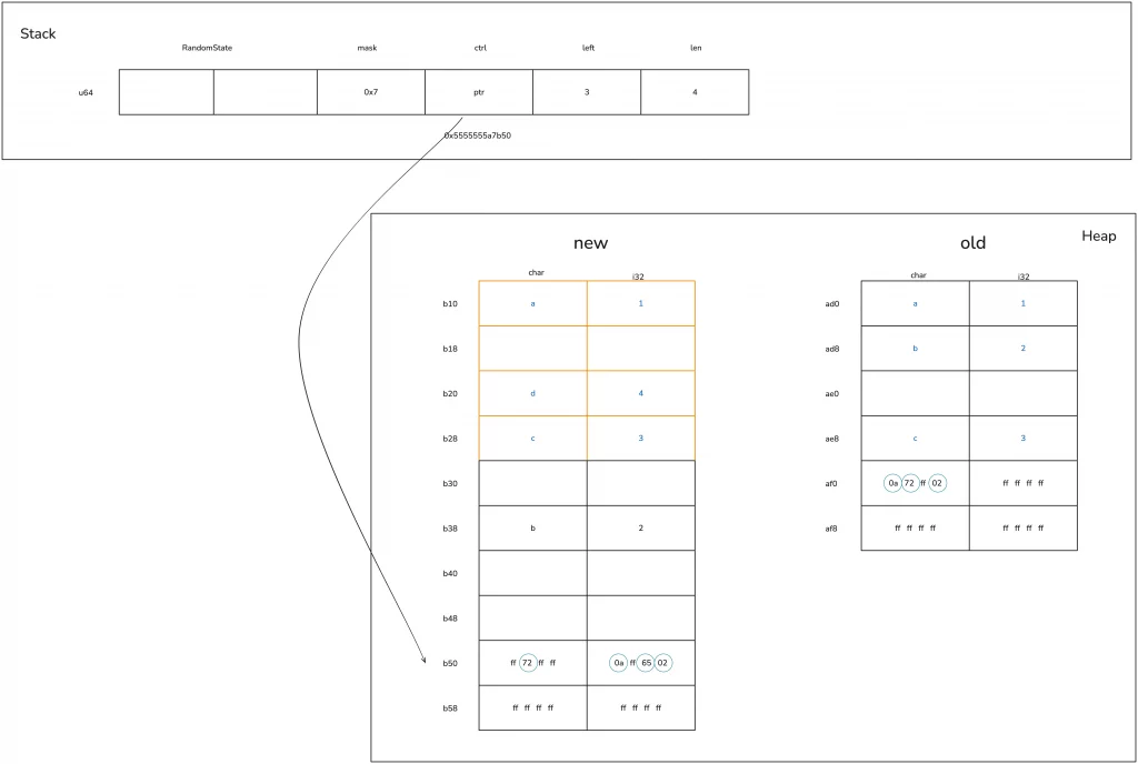
According to the information obtained from rust-gdb, let’s see how the hash table, which has no remaining space after inserting three elements, grows when adding ’d’: 4.
First, the hash table expands by a power of two, increasing from 4 buckets to 8 buckets.
This leads to the allocation of new heap memory, and then the original ctrl table and corresponding key-value data are moved to the new memory. In this example, because char and i32 implement the Copy trait, it’s a copy operation; if the key type were String, only the 24-byte structure (ptr|cap|len) of the String would be moved, and the actual memory of the String would not need to change.
During the moving process, hash reallocation is involved. As shown in the figure below, you can see that the relative positions and their ctrl bytes for ‘a’ / ‘c’ haven’t changed, but after recalculating the hash, the ctrl byte and position of ‘b’ have changed:
Deleting a value
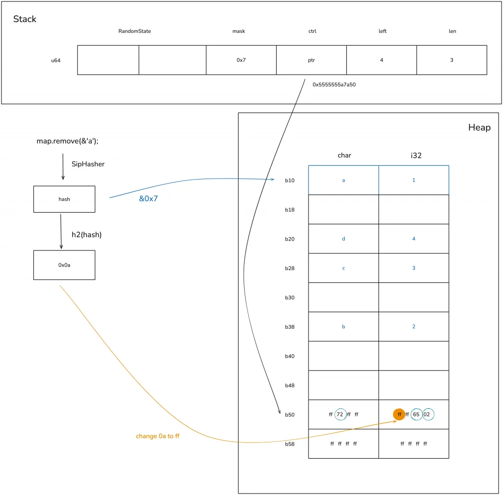
Now that we understand how the hash table grows, let’s look at what happens when deleting a value.
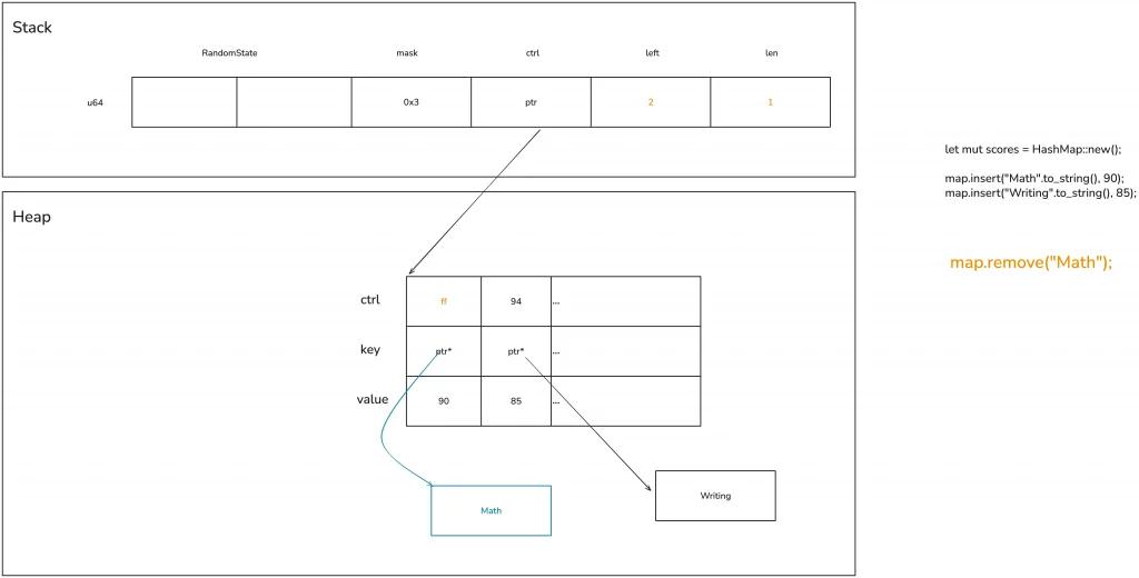
When you want to delete a value from the hash table, the process is similar to searching: you first need to find the position of the key to be deleted. After finding the specific location, there’s no need to actually clear the memory; you only need to set its ctrl byte back to 0xff (or mark it as deleted). This way, this bucket can be reused again:
There is an issue here: when the key/value has additional memory, such as String, its memory is not immediately reclaimed. Only the next time the corresponding bucket is used, when the HashMap no longer owns this String, is the String’s memory reclaimed. Let’s look at the schematic diagram below:
There is an issue here: when the key/value has additional memory, such as String, its memory is not immediately reclaimed. Only the next time the corresponding bucket is used, when the HashMap no longer owns this String, is the String’s memory reclaimed. Let’s look at the schematic diagram below:
Generally, this doesn’t cause major problems, at most resulting in slightly higher memory usage. However, in some extreme cases, such as running after adding a large amount of content to the hash table and then deleting a large amount of content, you can release the unnecessary memory using shrink_to_fit / shrink_to.
Allow custom data structures to serve as hash keys
Sometimes, we need custom data structures to be keys in a HashMap. This requires the use of three traits: Hash, PartialEq, and Eq, all of which can be automatically derived via derive macros. Among them:
- implementing
Hashallows the data structure to compute a hash; - implementing
PartialEq/Eqallows the data structure to be compared for equality and inequality.Eqimplements reflexivity (a == a), symmetry (if a == b then b == a), and transitivity (if a == b and b == c, then a == c), whilePartialEqdoes not implement reflexivity.
We can write an example to see how custom data structures can support this:
use std::{
    collections::{HashMap, hash_map::DefaultHasher},
    hash::{Hash, Hasher},
};

#[derive(Debug, Hash, PartialEq, Eq)]
struct Student<'a> {
    name: &'a str,
    age: u8,
}

impl<'a> Student<'a> {
    pub fn new(name: &'a str, age: u8) -> Self {
        Self { name, age }
    }
}

fn main() {
    let mut hasher = DefaultHasher::new();
    let student = Student::new("Qwe", 18);

    student.hash(&mut hasher);
    let mut map = HashMap::new();

    map.insert(student, vec!["Math", "Writing"]);
    println!("hash: 0x{:x}, map: {:?}", hasher.finish(), map);
}
HashSet / BTreeMap / BTreeSet
Finally, we briefly discuss several other data structures related to HashMap.
Sometimes we only need to simply confirm whether an element is in a set, and using HashMap would be a waste of space. In such cases, HashSet can be used, which is a simplified version of HashMap and can be used to store unordered sets. Its definition is directly HashMap<K, ()>:
use hashbrown::hash_set as base;

pub struct HashSet<T, S = RandomState> {
    base: base::HashSet<T, S>,
}

pub struct HashSet<T, S = DefaultHashBuilder, A: Allocator + Clone = Global> {
    pub(crate) map: HashMap<T, (), S, A>,
}
Using HashSet to check if an element belongs to a set is highly efficient.
Another commonly used data structure alongside HashMap is BTreeMap. BTreeMap is a data structure that internally uses a B-tree to organize the hash table. Additionally, BTreeSet is similar to HashSet and is a simplified version of BTreeMap, used to store ordered sets.
Here, we focus on BTreeMap, whose data structure is as follows:
pub struct BTreeMap<K, V> {
    root: Option<Root<K, V>>,
    length: usize,
}

pub type Root<K, V> = NodeRef<marker::Owned, K, V, marker::LeafOrInternal>;

pub struct NodeRef<BorrowType, K, V, Type> {
    height: usize,
    node: NonNull<LeafNode<K, V>>,
    _marker: PhantomData<(BorrowType, Type)>,
}

struct LeafNode<K, V> {
    parent: Option<NonNull<InternalNode<K, V>>>,
    parent_idx: MaybeUninit<u16>,
    len: u16,
    keys: [MaybeUninit<K>; CAPACITY],
    vals: [MaybeUninit<V>; CAPACITY],
}

struct InternalNode<K, V> {
    data: LeafNode<K, V>,
    edges: [MaybeUninit<BoxedNode<K, V>>; 2 * B],
}
Unlike HashMap, BTreeMap is ordered. Let’s look at an example:
use std::collections::BTreeMap;

fn main() {
    let map = BTreeMap::new();
    let mut map = explain("empty", map);

    for i in 0..16usize {
        map.insert(format!("Qwe {}", i), i);
    }

    let mut map = explain("added", map);

    map.remove("Qwe 1");

    let map = explain("remove 1", map);

    for item in map.iter() {
        println!("{:?}", item);
    }
}


fn explain<K, V>(name: &str, map: BTreeMap<K, V>) -> BTreeMap<K, V> {
    let arr: [usize; 3] = unsafe { std::mem::transmute(map) };
    println!(
        "{}: height: {}, root node: 0x{:x}, len: 0x{:x},",
        name, arr[1], arr[0], arr[2]
    );
    unsafe { std::mem::transmute(arr) }
}
Its output is as follows:
empty: height: 0, root node: 0x0, len: 0x0,
added: height: 1, root node: 0x102b66a30, len: 0x10,
remove 1: height: 1, root node: 0x102b66a30, len: 0xf,
("Qwe 0", 0)
("Qwe 10", 10)
("Qwe 11", 11)
("Qwe 12", 12)
("Qwe 13", 13)
("Qwe 14", 14)
("Qwe 15", 15)
("Qwe 2", 2)
("Qwe 3", 3)
("Qwe 4", 4)
("Qwe 5", 5)
("Qwe 6", 6)
("Qwe 7", 7)
("Qwe 8", 8)
("Qwe 9", 9)
It can be seen that during traversal, BTreeMap prints the values in the order of the keys. If you want a custom data structure to be usable as a key in BTreeMap, then you need to implement PartialOrd and Ord. The relationship between these two is similar to that of PartialEq / Eq, and PartialOrd also does not implement reflexivity. Similarly, PartialOrd and Ord can also be implemented via derive macros.
Summary
In learning data structures, you must clearly understand the memory layout and basic algorithms of commonly used data structures, and try to have a good idea of how they grow under different circumstances.